Measuring exactly how long a program requires to run or how much memory it consumes is challenging, because the results depend upon many details of how a computer is configured. A more reliable way to characterize the efficiency of a program is to measure how many times some event occurs, such as a function call.

Let's return to our first tree-recursive function, the fib function for computing numbers in the Fibonacci sequence.

>>> def fib(n):
            if n == 0:
                return 0
            if n == 1:
                return 1
            return fib(n-2) + fib(n-1)
    

>>> fib(5)
    5
    

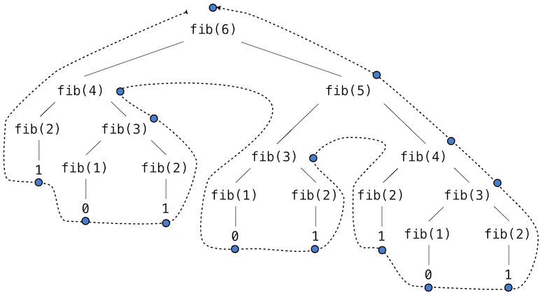
Consider the pattern of computation that results from evaluating fib(6), depicted below. To compute fib(5), we compute fib(3) and fib(4). To compute fib(3), we compute fib(1) and fib(2). In general, the evolved process looks like a tree. Each blue dot indicates a completed computation of a Fibonacci number in the traversal of this tree.

This function is instructive as a prototypical tree recursion, but it is a terribly inefficient way to compute Fibonacci numbers because it does so much redundant computation. The entire computation of fib(3) is duplicated.

We can measure this inefficiency. The higher-order count function returns an equivalent function to its argument that also maintains a call_count attribute. In this way, we can inspect just how many times fib is called.

>>> def count(f):
            def counted(*args):
                counted.call_count += 1
                return f(*args)
            counted.call_count = 0
            return counted
    

By counting the number of calls to fib, we see that the calls required grows faster than the Fibonacci numbers themselves. This rapid expansion of calls is characteristic of tree-recursive functions.

>>> fib = count(fib)
    >>> fib(19)
    4181
    >>> fib.call_count
    13529
    

Space. To understand the space requirements of a function, we must specify generally how memory is used, preserved, and reclaimed in our environment model of computation. In evaluating an expression, the interpreter preserves all active environments and all values and frames referenced by those environments. An environment is active if it provides the evaluation context for some expression being evaluated. An environment becomes inactive whenever the function call for which its first frame was created finally returns.

For example, when evaluating fib, the interpreter proceeds to compute each value in the order shown previously, traversing the structure of the tree. To do so, it only needs to keep track of those nodes that are above the current node in the tree at any point in the computation. The memory used to evaluate the rest of the branches can be reclaimed because it cannot affect future computation. In general, the space required for tree-recursive functions will be proportional to the maximum depth of the tree.

The diagram below depicts the environment created by evaluating fib(3). In the process of evaluating the return expression for the initial application of fib, the expression fib(n-2) is evaluated, yielding a value of 0. Once this value is computed, the corresponding environment frame (grayed out) is no longer needed: it is not part of an active environment. Thus, a well-designed interpreter can reclaim the memory that was used to store this frame. On the other hand, if the interpreter is currently evaluating fib(n-1), then the environment created by this application of fib (in which n is 2) is active. In turn, the environment originally created to apply fib to 3 is active because its return value has not yet been computed.

The higher-order count_frames function tracks open_count, the number of calls to the function f that have not yet returned. The max_count attribute is the maximum value ever attained by open_count, and it corresponds to the maximum number of frames that are ever simultaneously active during the course of computation.

>>> def count_frames(f):
            def counted(*args):
                counted.open_count += 1
                counted.max_count = max(counted.max_count, counted.open_count)
                result = f(*args)
                counted.open_count -= 1
                return result
            counted.open_count = 0
            counted.max_count = 0
            return counted
    

>>> fib = count_frames(fib)
    >>> fib(19)
    4181
    >>> fib.open_count
    0
    >>> fib.max_count
    19
    >>> fib(24)
    46368
    >>> fib.max_count
    24
    

To summarize, the space requirement of the fib function, measured in active frames, is one less than the input, which tends to be small. The time requirement measured in total recursive calls is larger than the output, which tends to be huge.